There are few things quite as satisfying as fixing your position by measuring the altitude of a few heavenly bodies. With no other landmarks around, stars and planets help to put a face on an otherwise featureless expanse of ocean — they become our friends at sea during the night. Even though there may no longer be a pressing need to use celestial navigation in the age of GPS, it seems a good way to stay in touch with our “friends.”
For the recreational navigator, the beauty of celestial navigation often becomes obscured by a maze of numbers and a lack of confidence. In this article, we introduce a few pragmatic tweaks to the old art, putting the focus back on those friendly stars and our sextant. Why not get more fun and insight out of practicing celestial navigation on board while mastering a new skill?
The approach we outline below can be applied to any celestial sight. It is particularly useful for fixing your position by observing multiple stars or planets at twilight. While the good old sun sight certainly has its value, there is a special reward in the instant gratification of finding your position without the uncertainties of a running fix.
Setting the focus
One way to make the process easier is to use one of the countless electronic calculators that reduces sight reduction to a few keystrokes and to focus our attention on taking and evaluating sights.
So, let’s take advantage of these modern tools to minimize the time spent on sight reduction and instead focus on taking and evaluating sights. The key to mastering celestial navigation is perfecting our ability to take accurate sights with our sextant. This takes practice on a rolling boat. The more of these measurements we can take and evaluate, the better. If you’d rather stick with the old pencil and paper method, there is nothing wrong with that — just don’t let it deter you from practicing and evaluating your sights!
Changing the game
To get a fix on our position, we need at least two intersecting lines of position (LOPs). Just doing the bare minimum — taking one sight each of two different bodies — leaves us exposed to a potentially large error in our fix because our sights may be far from perfect. To improve our fix, we could take additional sights of other bodies that would add LOPs to our plot. The more LOPs we have, the better we can box in our position, or so the argument goes. However, for us recreational practitioners, the accuracy of our individual sights often remains uncertain. Additional LOPs may actually increase ambiguity rather than confidence in our fix. Fixing our position inside (and in some cases outside) the cocked hat becomes guesswork, making it difficult to systematically identify and learn from our mistakes.
An alternative to adding more LOPs in order to increase confidence in our fix is to stick with only two LOPs but try to make these as accurate as possible. How do we do that? We know that our sights will not be perfect. They will include an unknown random error; some will be too high, others too low. For a single measurement it will be impossible to tell which and by how much. However, if we had a series of altitude measurements of the same body, we could obtain a better estimate of its true altitude (and therefore a high-quality LOP) by applying simple statistical methods. So let’s stick with two bodies and use those precious minutes of twilight to take multiple sights of each.
 |
|
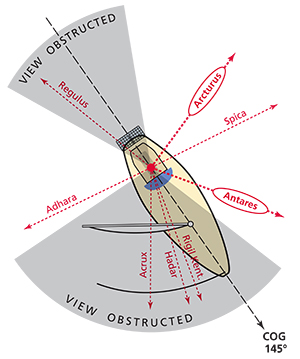
When attempting star sights, some stars will be obstructed by sails or gear, others won’t be bright, others won’t yield a good crossing angle. In this case the best stars are Arcturus and Antares. |
How do we combine these multiple measurements to obtain a good estimate of the true altitude of each body? Intuitively, we think of the average (arithmetic mean) as a way to cancel out errors in a series of measurements. It turns out that this is not the best method for sextant sights taken on a small boat though. Here, we’re in the realm of what statisticians call “non-parametric estimation,” and for this case, a much better and simpler estimator of the true altitude value is the median, the middle value out of a sorted series of measurements. The median is robust and well suited for situations where we cannot make assumptions about the statistical properties of our measurements — precisely what we need.
With this in mind, the approach we propose is straightforward:
Step 1: Identify two bodies (stars, planets, moon) that will be visible at twilight, with their azimuth angles separated by 45 to 135 degrees (90° ± 45°). A difference in azimuths outside this range will lead to an LOP crossing angle that is either too acute or too obtuse and may amplify any error in the altitude measurement when later plotting the fix. For example, one June evening found us sailing our 35-foot sloop Namani between Fiji’s Lau islands. Looking for suitable candidates among the 57 navigational stars, we selected bright stars that would be visible above the horizon. This left us with eight stars. Of these eight, only four were not obscured by sails or rigging and gear off the stern, and only Arcturus and Antares provided a robust crossing angle — another very good reason to focus on only two bodies.
Step 2: At twilight, take an odd number of sights for each of the two bodies in quick succession. Five sights each works well. We have found little improvement from taking seven or more sights.
Step 3: Use your preferred method for calculating the intercept for each sight (10 intercept values if you took five sights of each of the two bodies). An electronic sight reduction tool will help do this quickly and easily.
Then, for each body, sort the intercept values and take the sight with the median (middle) intercept value to plot the LOP. For example, if the sights of one of our two observed bodies yielded a sorted intercept series of 4.2 away, 3.9 away, 1.2 away, 0.3 toward and 2.8 toward, we would take the middle value of 1.2 away and its associated azimuth angle to plot the LOP for this body.
Step 4: Plot the two LOPs to determine the fix latitude and longitude. Some electronic calculators will do this automatically.
 |
|
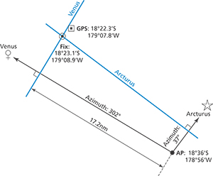
In Figure 1 we see a fix from the intersection of lines of position from sights of Venus and Arcturus. |
Step 5: Evaluate your fix against your GPS position, looking for ways to improve your sights by reducing any systematic error in your measurements (more on that later).
In addition to providing robust estimates of the observed bodies’ true altitudes and thus high-quality LOPs, this approach also allows us to collect a comprehensive set of sight data. We can later analyze this data to help us improve the quality of our sights.
Five sights each for two bodies may sound like a lot, but it is actually quite quick and easy. Since we stick with the same star or planet for each sight series, we don’t have to reset the sextant and bring the body all the way down to the horizon every time. Nor do we have to change our orientation or our position on the boat, and the software eliminates the work of manually reducing the 10 sights.
Putting it all together
For a complete example, let’s go back to that June evening in Fiji: an overnight passage, the sun setting to the west and a mostly cloudless sky. With beam reaching on a course of 145 degrees at evening twilight, we were lucky to have Venus available for a sight. Figure 5 shows the five sights we took of Venus, sorted by intercept.
Our second sight landed on the median position with an intercept of 17.2 toward. Since we had a GPS position to later check our fix, we could also calculate the theoretically correct intercept of 16.8 toward. This made our median sight 0.4 too high but significantly better than the first, third and fourth sights. As it turned out, the fifth sight was even closer to the true value, although we would have had no way of knowing that without peeking at the GPS. Our objective here is not to identify the best sight in our series, which would be impossible without GPS, but to have a method that will reliably produce a good estimate of the true altitude value. Most importantly, it will eliminate outliers such as the first and third sights. Had we only taken one sight, our LOP would have been off by 1.8 nm (sight number 1) rather than 0.4 nm and, without knowledge of our GPS position, we would have had no way of judging the quality of that single sight.
The example above also demonstrates that the first and third sights skew the mean (average) intercept (as opposed to the median intercept) upward to 17.5 nm. Scenarios like this, where the outliers are distributed asymmetrically around the true value, are quite common with waves rolling the boat and obscuring the horizon. In these cases, taking the median sight will produce better results than using the mean of a series.
The complete fix from our example is shown in an accompanying diagram, with the second LOP derived from a five-sight series of Arcturus.
 |
|
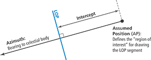
Figure 2 shows the relationship between the assumed position, the intercept and the LOP. |
Some fine-tuning
As recreational practitioners of celestial navigation, we could stop here and already have a robust and pragmatic method for producing reliable fixes. But while we’re at it, we may as well push the idea a little further.
One thing to keep in mind when applying the above procedure is that our position changes over the course of the sights, effectively producing a running fix over a short distance. In most cases, we will not be concerned about the small error this introduces. For example, if our first and our last sight were taken 20 minutes apart at a boat speed of 6 knots, the resulting intercept error for a star that was observed 60 degrees forward or aft of the beam would be 1.7 nautical miles at most — unlikely to bother us on the open ocean. The error will be less for bodies that lie closer to the beam. Swifter work will reduce this error; 20 minutes is a generous allowance for completing the two sight series.
If we wanted to eliminate this error, we can borrow a page from aviators for whom this is a more substantial issue. Sight Reduction Tables for Air Navigation (No. 249 Volume 1) includes a handy table to correct a calculated intercept for “Motion of the Observer.” The navigator enters the table with speed over ground (SOG) and the relative angle that a bearing line to the observed body forms with the ship’s course over ground (COG). Given these two arguments, the table provides the correction to be applied to our calculated intercept per minute of elapsed time. At 50 to 900 knots, the SOG for which these corrections are tabulated is more representative of aircraft than of cruising sailboats. We can, however, simply divide the SOG values and the resulting corrections by 10 or 100 to match our earthbound realities (look for “Alternative Table 1” at the end of the publication).
Some electronic sight reduction calculators (such as the CelNav package detailed in the sidebar) will automatically correct for this error. We also find this correction convenient to advance or delay our celestial fixes to fall on the half-hour, making them easier to reconcile with the ship’s dead reckoning plot.
Another aspect to keep in mind is systematic error. Possible causes for systematic error include a misaligned sextant, misjudging the horizon in a big swell or failing to swing the sextant correctly to measure the exact shortest distance between the observed body and the horizon. Picking the median intercept will help reduce random error in our sights but not a systematic error. While our method cannot compensate for such systematic errors, the data we collect in the process can help us identify and remedy them. Assuming we are practicing celestial navigation for our own enjoyment and still have access to GPS data, we can use our GPS position at the time of the fix as our assumed position (AP) for the sight reduction calculation (when using a celestial calculator). If our sights were perfect, our intercepts would come out at zero, resulting in an LOP that runs through our GPS position. We can then immediately tell from our intercept values whether our sight series appears to be shifted consistently above or below zero rather than being scattered around this central value. If we spot such a bias, we can track down the root cause and start to correct for it, successively perfecting our technique.
Early into a four-week passage between the Galapagos Islands and the Marquesas, one of us found his sights to be “high” by one to two arc minutes on average. After carefully checking the sextant and eliminating misalignment as a possible error source, the problem was eventually tracked down to gripping the sextant too tightly, resulting in a skewed swinging motion. This, in turn, led to systematically overstated altitude readings. Loosening the grip — after adding a wrist-loop to allay our fear of losing the precious piece overboard — showed an immediate and permanent improvement in sight accuracy. The ability to easily spot these biases is also the main reason why we use a sorted series of intercepts rather than simply picking the median among fully corrected sextant altitudes, which would save us eight subtractions in the process.
Another valuable exercise is to mark the best-perceived sight in each series and then check the actual accuracy based on the GPS position. It took us a while to figure out what makes a “good sight,” but in the process we learned to judge the quality of our sights as we take them. This becomes particularly valuable when we have to make do with a single sight, snuck in between the clouds, without the luxury of a full five-sight series.
 |
|
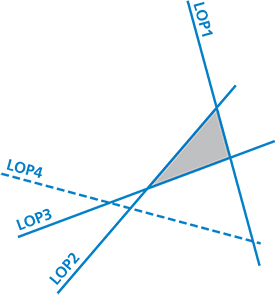
In Figure 3 we see a fix from crossing LOP 1, 2 and 3. LOP 4 is discarded. |
Wrapping up
To recap: We focus on the essence of celestial navigation by letting electronic tools automate the tedious sight reduction procedure. Then, instead of using LOPs from many different bodies, we take a short series of sights of only two bodies. Applying the median estimator to the resulting data improves our fix accuracy by reducing random error and the impact of outliers. It also provides valuable feedback for improving our technique by identifying and eliminating systematic errors.
With this approach, we recreational navigators get about 80 percent of our fixes within four nautical miles of our GPS position and 97 percent within 10 nautical miles. The method proves particularly useful in higher seas with a pronounced rolling of the boat. While the spread of the intercept values increases in higher seas, the median has remained surprisingly robust in our experience.
Perhaps the biggest benefit has been the confidence we developed in our sight-taking and our ability to judge the quality of our sights. As a result, a sometimes-frustrating “trial and error” experience has become a fun pastime in which we can actually see our progress.
The ultimate reward comes when we can switch off the GPS and experience the satisfaction of practicing an old art on our small boat. And who knows? Now that we’ve got the important parts down, we may even turn purist and dig out those sight reduction tables again…
Markus Schweitzer worked in the tourism, logistics and aviation industries before casting off the shorelines. He, his wife and young son recently returned from a three-year trans-Pacific journey aboard their 35-foot sloop Namani. His background is in engineering and computational mathematics. You can follow Namani’s travels at www.namaniatsea.org.
William Noonan is a physicist at John Hopkins University Applied Physics Laboratory. He has joined Namani’s crew on numerous passages in the Atlantic and Pacific Oceans. As a life-long sailor he enjoys his time aboard Namani as an opportunity to practice his celestial navigation skills and to bring some scientific rigor to the old art.